Nonlinear Regression Reference

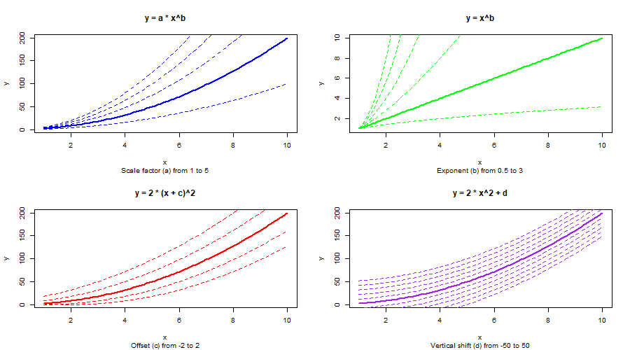
Fitting nonlinear utility functions comes up regularly for data interpolation. There are a handful of useful functional forms that can be implemented to match the approximate shape of a given dataset. Often we jump to the default options in Microsoft Excel (exponential, linear, logarithmic, polynomial, or power), but there are many other shapes that can often provide a better fit to the relationship. Unfortunately, neither R or Excel provide an easy visual reference to find the desired shape. They also don't make it easy to manipulate the functions. The goal of this blog post is to provide a quick visual reference for various nonlinear functions. Examples are provided in R and links from Desmos (https://www.desmos.com/) are provided to play around with the parameters to see the flexibility of the shape of the relationships.

Polynomial Functions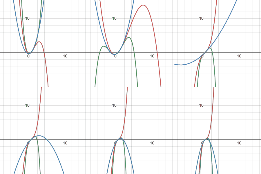

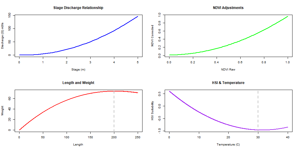
Edit function on Desmos

Polynomials are useful to fit simple relationships. It is best to use them for interpolation rather than extrapolation given bizarre behavior outside of the fitted data range. This is especially true for high degree polynomials. For example see the length and weight relationship in the example below. If you are trying to fit a complex relationship with a polynomial function it is best to develop multiple polynomial function for a range of data on the x-axis rather than a global function. Polynomial functions are also linear (or can be transformed to be linear) for simple fitting lm(y ~ x + I(x^2) + I(x^3))in R. Normalizing the data can help to prevent extreme coefficients from model fitting.

y = (2.5*x)^2 - (1.8*x) + 0.2 # Stage and discharge

y = (0.95*x)^2 + (0.05*x) + 0.01 # NDVI correction

y = (0.012*x)^3 - (0.05*x)^2 + (0.8*x) # Length and weight

y = (-0.005*x)^3 + (-0.04*x)^2 + (-0.1*x) + 0.6 # HSI & Temperature

Power Law Functions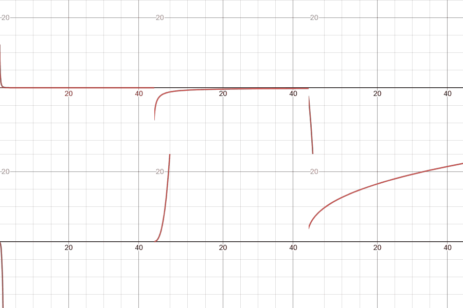

Edit function on Desmos

Generally, either a one-term (y = ax^b) or two-term (y = ax^b + c) functional form. Possible applications:

• Hydrology:
  • Describes river discharge as a function of drainage area or flow velocity vs. channel slope (Q = ax^b).
• Remote Sensing:
  • Models the relationship between reflectance and surface roughness.
• Population ecology:
  • Fish weight-length relationships (Weight = a * (Length^b)).
• General Ecology:
  • Allometric scaling laws (e.g., metabolic rates vs. body size).

y <- 0.5 * x^0.8

y <- 2 * x^(-1.2)

y <- 0.01 * x^3

y <- 0.3 * x^0.75

Exponential Function

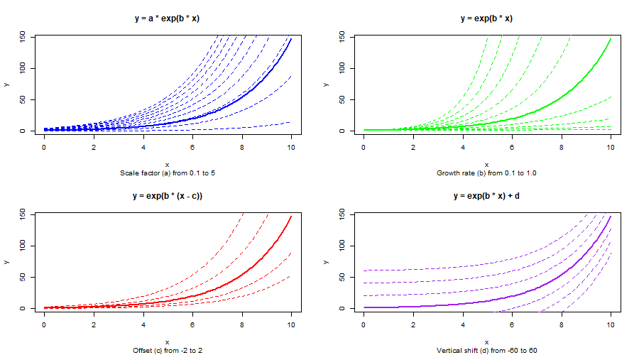
Potential applications include modelling rainfall decay over time in infiltration studies, exponential population growth/decay etc.

y = a*e^(0.5*x)

• Scaling the Curve (a):
  • Adjusting a changes the overall magnitude of the curve.
  • Example: y=a*e^(0.5*x)
• Changing the Growth Rate (b):
  • Modifying b controls how steeply the curve grows (or decays if b<0).
  • Example: y=e^(b*x)
• Adding an Offset to x:
  • Introducing c shifts the curve along the x-axis, effectively changing the starting point of growth.
  • Example: y=e^(0.5*x-c))
• Applying a Vertical Shift (d):
  • Adding d shifts the entire curve up or down along the y-axis without altering its growth rate.
  • Example: y=e^(0.5*x) + d.

Hyperbolic Function

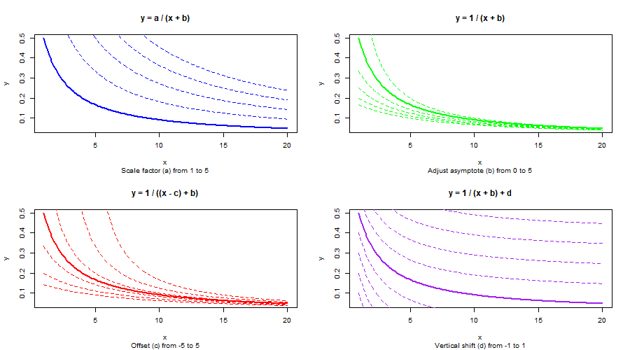
y=(a/(x+b))

Logarithmic Function

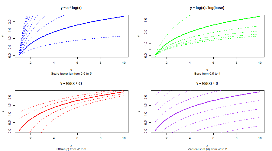
y=log(x)

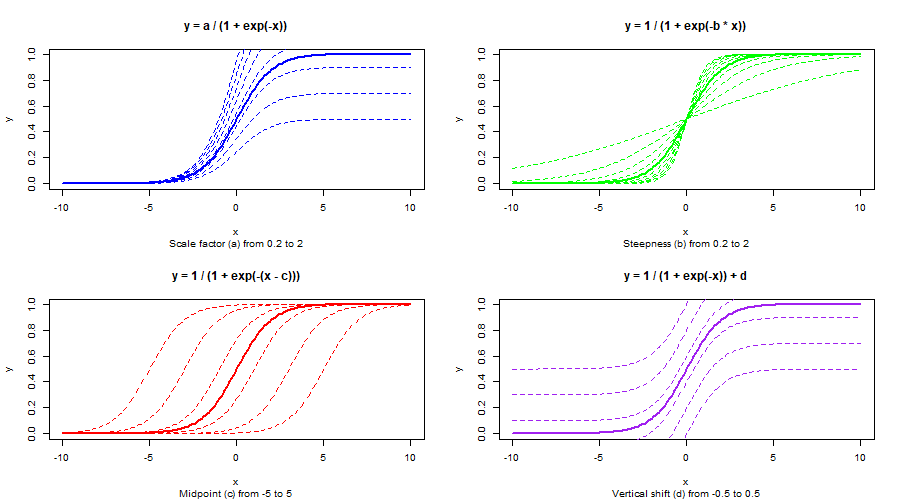
Logistic Function

y=1/(1 + exp(-1*(x-2)))

y=a/(1 + exp(-b*(x-c)))

a = the curve's maximum value
b = logistic growth rate or steepness of the curve
c = the x value of the sigmoid midpoint

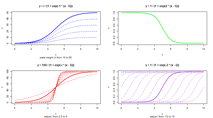
Sigmoid Function

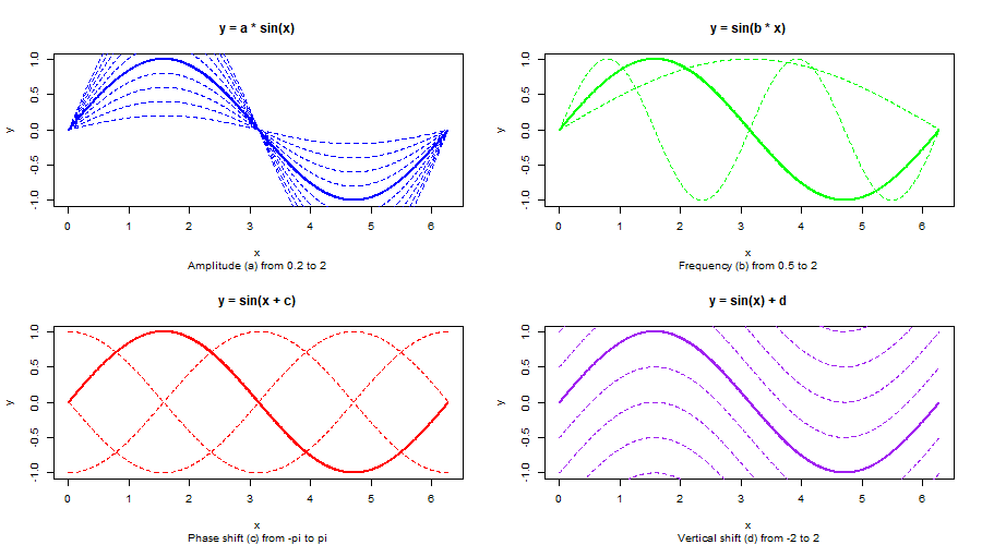
Sine Curve

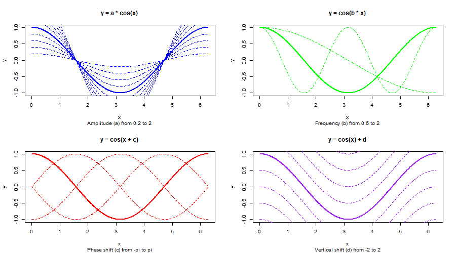
Cosine Curve

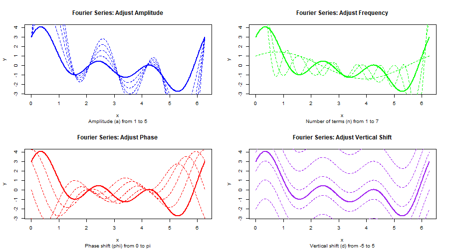
Fourier Series

First define function:

fourier_series <- function(x, n_terms = 5, a = 1, b = 1) {
 y <- 0
 for (n in 1:n_terms) {
   y <- y + a * sin(n * x) + b * cos(n * x)
 }
 return(y)
}

x <- seq(0, 2 * pi, by = 0.01)
y <- fourier_series(x, n_terms = 3, a = 1, b = 1)
plot(x, y, type = "l")

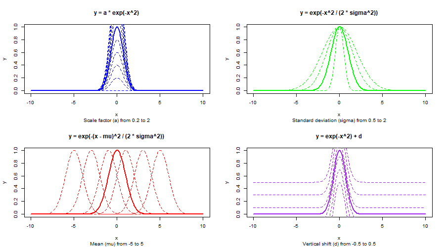
Gaussian Curve