Sediment and Westslope Cutthroat Trout
mbakken
View all records in the stressor response library

Species Common Name
Westslope Cutthroat Trout
Latin Name (Genus species)
Oncorhynchus clarkii lewisi
Stressor Name
Sediment increase
Specific Stressor Metric
Relative increase in sediment from background
Stressor Units
Unitless
Vital Rate (Process)
System capacity
Geography
Alberta foothills watersheds, excluding National Parks
Detailed SR Function Description
Sedimentation can reduce the biological productivity of aquatic ecosystems and damage fish habitat (GOA 2023). The amount of sediment a stream can transport is based on numerous factors including, but not limited to, precipitation, surface water transport, erosion, topography, geology and riparian vegetation (reviewed in Muck 2010). Anthropogenic disturbances (e.g., such as roads, Lachance et al. 2008) can produce substantial inputs of sediments into streams in excess of natural levels. These increased rates of sediment delivery can adversely affect bull trout habitat and have lethal and sub-lethal effects throughout trout life history from egg incubation to adulthood (reviewed in Muck 2010).
Potential impacts caused by excessive suspended sediments are varied, complex and often masked by other concurrent activities (Newcombe 2003), making it difficult to establish the specific effects of sediment impacts on fish (Chapman 1988). The sediment stressor-response curve was developed using sediment estimates obtained from ALCES online based on 2010 footprint and current FSA risk categories for the native trout species (see MacPherson et al. 2019; AEP 2013, 2018, 2019) in the HUC 8 watersheds across Alberta’s East Slopes. FSA risk categories vary from 0 (functionally extirpated) to 5 (very low risk). The dynamic pattern of sediment transport varies from watershed to watershed and aquatic ecosystems have adapted to the natural temporal and spatial pattern of this transport. As such, effects on fish from changes in sediment loading will be relative to natural conditions (Kemp et al. 2011). To capture relative change, sediment in the stressor-response curve was defined as the “sediment index” which is measured as potential sediment loading for 2010 (tonnes/ha/year) divided by potential sediment loading for 1910 (tonnes/ha/year).
The sediment index (2010 loading/1910 loading) stressor-response curves were derived by: a) using logistic regression to develop a statistical model relating probability of being within a given FSA category to the log-transformed sediment index; and, b) converting this statistical model into a stressor-response curve relating sediment to the system capacity of the 3 trout species. Proportional-odds logistic regression was used as the response variable is a multinomial ordered variable (Venables and Ripley 2002). The proportional-odds assumption of independence among adjacent categories was assessed by comparing similarity of odds ratios among successive categories (Venables and Ripley 2002).
The stressor-response curve was derived from the proportional-odds logistic-regression models by estimating sediment index levels required for a 90% probability of falling within a given FSA category. This is similar logic to quantile regression (Cade and Noon 2003) that recognizes numerous unaccounted factors can be driving a response variable. FSA categories were converted to percent of reference condition using population percentages at transition points between adjacent FSA categories.
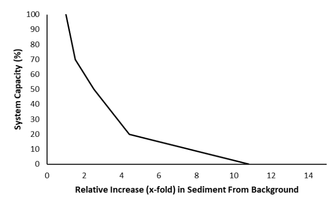
Compared to phosphorus, the data showed a much clearer separation among FSA categories with increasing sediment relative to background 1910 values. An adult FSA category of 4 existed in watersheds when relative sediment increases were negligible. FSA categories of 1 or 0 dominated when sediment increased more than 3-fold over background levels. Not surprisingly, there was a significant and strong negative sediment effect on association with FSA categories (slope = -2.8, 95% profile confidence interval –3.8 to -2.0). The stressor-response curve is shown in Figure 1.
A major issue in assessing the importance of potential stressors in driving a response variable is collinearity amongst different stressors (Zuur et al. 2010). If different stressors are highly correlated, it is impossible to distinguish relative importance without further experimentation. There was a high degree of correlation between potential phosphorus loading (tonnes/ha/year) and the relative sediment increase across the 73 watersheds (Pearson R = 0.62, 95% confidence interval 0.45 – 0.74). Thus, it was difficult using the available data to separate the importance of phosphorus or sediment independently on system capacity. Our approach was to create two separate stressor-response curves (i.e., one for potential phosphorus loading independent of the sediment index and vice-versa) and acknowledge that the observed response could be driven by the other stressor. As the Joe model accumulates cumulative effects multiplicatively (additive on a proportional scale), treating these two curves separately would inappropriately overemphasize the expected response. To overcome this issue, we treated sediment and phosphorus in the Joe model using a limiting factor approach. Simply, only the strongest, negative response from either the phosphorus or sediment stressor-response curves is used to calculate final system capacity. Anytime a watershed shows either phosphorus or sediment to be a hypothesized key driver, it must be acknowledged that the other stressor (i.e., sediment or phosphorus, respectively) could be the driver given the collinearity.
Potential impacts caused by excessive suspended sediments are varied, complex and often masked by other concurrent activities (Newcombe 2003), making it difficult to establish the specific effects of sediment impacts on fish (Chapman 1988). The sediment stressor-response curve was developed using sediment estimates obtained from ALCES online based on 2010 footprint and current FSA risk categories for the native trout species (see MacPherson et al. 2019; AEP 2013, 2018, 2019) in the HUC 8 watersheds across Alberta’s East Slopes. FSA risk categories vary from 0 (functionally extirpated) to 5 (very low risk). The dynamic pattern of sediment transport varies from watershed to watershed and aquatic ecosystems have adapted to the natural temporal and spatial pattern of this transport. As such, effects on fish from changes in sediment loading will be relative to natural conditions (Kemp et al. 2011). To capture relative change, sediment in the stressor-response curve was defined as the “sediment index” which is measured as potential sediment loading for 2010 (tonnes/ha/year) divided by potential sediment loading for 1910 (tonnes/ha/year).
The sediment index (2010 loading/1910 loading) stressor-response curves were derived by: a) using logistic regression to develop a statistical model relating probability of being within a given FSA category to the log-transformed sediment index; and, b) converting this statistical model into a stressor-response curve relating sediment to the system capacity of the 3 trout species. Proportional-odds logistic regression was used as the response variable is a multinomial ordered variable (Venables and Ripley 2002). The proportional-odds assumption of independence among adjacent categories was assessed by comparing similarity of odds ratios among successive categories (Venables and Ripley 2002).
The stressor-response curve was derived from the proportional-odds logistic-regression models by estimating sediment index levels required for a 90% probability of falling within a given FSA category. This is similar logic to quantile regression (Cade and Noon 2003) that recognizes numerous unaccounted factors can be driving a response variable. FSA categories were converted to percent of reference condition using population percentages at transition points between adjacent FSA categories.
Compared to phosphorus, the data showed a much clearer separation among FSA categories with increasing sediment relative to background 1910 values. An adult FSA category of 4 existed in watersheds when relative sediment increases were negligible. FSA categories of 1 or 0 dominated when sediment increased more than 3-fold over background levels. Not surprisingly, there was a significant and strong negative sediment effect on association with FSA categories (slope = -2.8, 95% profile confidence interval –3.8 to -2.0). The stressor-response curve is shown in Figure 1.
A major issue in assessing the importance of potential stressors in driving a response variable is collinearity amongst different stressors (Zuur et al. 2010). If different stressors are highly correlated, it is impossible to distinguish relative importance without further experimentation. There was a high degree of correlation between potential phosphorus loading (tonnes/ha/year) and the relative sediment increase across the 73 watersheds (Pearson R = 0.62, 95% confidence interval 0.45 – 0.74). Thus, it was difficult using the available data to separate the importance of phosphorus or sediment independently on system capacity. Our approach was to create two separate stressor-response curves (i.e., one for potential phosphorus loading independent of the sediment index and vice-versa) and acknowledge that the observed response could be driven by the other stressor. As the Joe model accumulates cumulative effects multiplicatively (additive on a proportional scale), treating these two curves separately would inappropriately overemphasize the expected response. To overcome this issue, we treated sediment and phosphorus in the Joe model using a limiting factor approach. Simply, only the strongest, negative response from either the phosphorus or sediment stressor-response curves is used to calculate final system capacity. Anytime a watershed shows either phosphorus or sediment to be a hypothesized key driver, it must be acknowledged that the other stressor (i.e., sediment or phosphorus, respectively) could be the driver given the collinearity.
Function Derivation
Landscape correlation
Transferability of Function
This function could be applied to any of the three species for which it was developed (Bull Trout, Athabasca Rainbow Trout, and Westslope Cutthroat Trout) within the Alberta range. While increased sedimentation has been shown to influence many aquatic systems, this function should be applied to other species with caution.
Source of stressor Data
The sediment index is calculated as the total expected sediment export for 2010 divided by the total expected sediment export before substantial industrial activity (i.e., 1910). Total expected sediment export was calculated following the Event Mean Concentration method described in Donahue (2013) and is based on land cover type and annual precipitation within the natural region. Sediment runoff values were obtained from the Upper Bow River Basin Cumulative Effects Study (ALCES, 2012) and sediment delivery coefficients were obtained from Stelfox et al. (2008). Delivery coefficients for OHV trails were assigned a value of 6% based on the work of Welsh (2008). Total estimated sediment export was calculated in ALCES Online © within the spatial unit of interest.
Function Type
continuous
Stressor Scale
linear
References Cited
Government of Alberta. 2024. Sediment stressor-response function for Athabasca Rainbow Trout, Westslope Cutthroat Trout, and Bull Trout. Environment and Protected Area Native Trout Cumulative Effects Model.
Alberta Environment and Parks (AEP). 2013. Bull Trout Fish Sustainability Index. Alberta Fish and Wildlife Policy Branch, Edmonton, Alberta. https://www.alberta.ca/bull-trout-fsi
Alberta Environment and Parks (AEP). 2018. Westslope Cutthroat Trout Fish Sustainability Index. Alberta Fish and Wildlife Policy Branch, Edmonton, Alberta. https://www.alberta.ca/westslope-cutthroat-trout-fsi
Alberta Environment and Parks (AEP). 2019. Athabasca Rainbow Trout Fish Sustainability Index. Alberta Fish and Wildlife Policy Branch, Edmonton, Alberta. https://www.alberta.ca/athabasca-rainbow-trout-fsi
ALCES 2012. Upper Bow River Basin Cumulative Effects Study. Report for Action for Agriculture, Alberta. 100 pp.
Chapman, D. W. 1988. Critical review of variables used to define effects of fines in redds of large salmonids. Transactions of the American Fisheries Society 117: 1-21
Donahue, W.F. 2013. Determining Appropriate Nutrient and Sediment Loading Coefficients for Modelling Effects of Changes in Landuse and Landcover in Alberta Watersheds. Water Matters Society of Alberta, Canmore, AB. 52pp.
Lachance, S., M. Dube, R. Dostie, and P. Berube. 2008. Temporal and spatial quantification of fine-sediment accumulation downstream of culverts in brook trout habitat. Transactions of the American Fisheries Society 137: 1826-1838
MacPherson, L., Sullivan, M., Reilly, J., and Paul, A. 2019. Alberta’s Fisheries Sustainability Assessment: A Guide to Assessing Population Status, and Quantifying Cumulative Effects using the Joe Modelling Technique. DFO Can. Sci. Advis. Sec. Res. Doc. 2019/058. vii + 45p
Muck. J. 2010. Biological effects of sedimentation on Bull Trout and their habitat – guidance for evaluating effects. U.S. Fish and Wildlife Service. Washington Fish and Wildlife Office. Lacey, WA
Newcombe, C. P. 2003. Impact assessment model for clear water fishes exposed to excessively cloudy water. Journal of the American Water Resources Association 39: 529-544
Stelfox, B., M. Anielski, M. Carlson, and T. Antoniuk. 2008. Alberta Southern East Slopes Integrated Land Management Pilot Project. Prepared for Alberta Environment and Alberta Sustainable Resource Development by the ASPEN Group. 55 p.
Venables, W. N., and B. D. Ripley. 2002. Modern Applied Statistics with S. Springer. https://doi.org/10.1007/978-0-387-21706-2_1
Welsh, M. J. 2008. Sediment Production and Delivery from Forest Roads and Off-Highway Vehicle Trails in the Upper South Platte River Watershed, Colorado. MSc thesis, Colorado State University
Zuur, A.F., E.N. Leno and C.S. Elphick. 2010. A protocol for data exploration to avoid common statistical problems. Methods in Ecology and Evolution 1:3-14
File Upload
Images
Stressor Response csv data
Data_WSCT_sediment.csv
(168 bytes)
| Sediment (x-fold increase from background) | Mean System Capacity (%) | SD | low.limit | up.limit |
|---|---|---|---|---|
| 1 | 100 | 0 | 0 | 100 |
| 1.5 | 70 | 0 | 0 | 100 |
| 2.5 | 50 | 0 | 0 | 100 |
| 4.4 | 20 | 0 | 0 | 100 |
| 10.8 | 0 | 0 | 0 | 100 |
Stressor Response Chart
Mean Response
±1 Standard Deviation
Upper/Lower Limits