canadaNHN - Canadian National Hydro Network R-package
Starting to put together some basic tools and functions in a new Canada NHN (National Hydrographic Network) R-package for interprovincial stream network summaries (https://github.com/mattjbayly/canadaNHN…) #hydrology #RStats #Canada #GIS
canadaNHN - Canadian National Hydro Network R-package
The Canadian National Hydrographic Network R-package is a collection of tools and functions designed to support the stream network analyses and watershed delineations from the Canadian NHN. Key functions include upstream and downstream network delineations from junction points as well as pseudo-watershed delineation based on RCA polygons.
Package Contributors:
Contributors include:
Features
- Upstream streamline network delineation from the NHN network
- Downstream streamline network delineation from the NHN network
- pseudo-RCA (each contributing areas) polygon generation
- Watershed delineation
Installation
The easiest way to install the canadaNHN package is from within the RStudio IDE using remotes::install_github(). At this time the package has not been published to CRAN so the default install.packages() will not work. Instead use remotes (or devtools) to install the packge directly from GitHub:
# You may need to install remotes library(remotes) remotes::install_github("mattjbayly/canadaNHN")
Usage
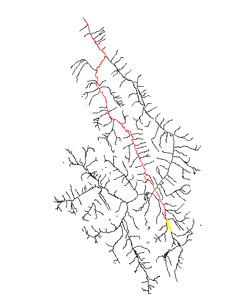
Trace downstream flow lines from a point
Trace the downstream flow path from an NHN junction nid (layer: NHN_HN_HYDROJUNCT_0). Inputs include the streamline vector layer (NHN_HN_NLFLOW_1) and a target junction nid as jnid.
# Your R code here
# Your R code here
# Load the iris dataset data(iris)
# Calculate the mean of the Sepal.Length column
mean_sepal_length <- mean(iris$Sepal.Length) print(paste("Mean Sepal Length:", mean_sepal_length)) # Create a histogram of the Sepal.Length column hist(iris$Sepal.Length, main = "Histogram of Sepal Lengths", xlab = "Sepal Length", col = "blue", border = "black")
# Load example data
filename_strm <- system.file("extdata", "NHN_HN_NLFLOW_1.gpkg", package = "canadaNHN")
``{r} # Your R code here
# Load example data
filename_strm <- system.file("extdata", "NHN_HN_NLFLOW_1.gpkg", package = "canadaNHN")
strm <- sf::st_read(paste0(filename_strm), layer="NHN_HN_NLFLOW_1") strm <- sf::st_zm(strm) #Trace downstream path target_junction_nid <- "484667c6025244219cfa5e5ee994715b" ds_lines <- get_downstream_lines(strm = strm, jnid = target_junction_nid, ds_sreach = 1000) plot(sf::st_geometry(strm)) plot(sf::st_geometry(ds_lines), add = TRUE, col = "red") out_sl <- strm[strm$fromJunction == target_junction_nid, ] plot(sf::st_geometry(out_sl), add = TRUE, col = "yellow", lwd = 4)
```
Trace upstream flow lines from a point
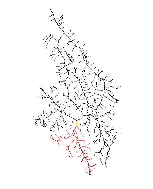
Trace all upstream flow paths from an NHN junction nid (layer: NHN_HN_HYDROJUNCT_0). Inputs include the streamline vector layer (NHN_HN_NLFLOW_1) and a target junction nid as jnid.
# Load example data filename_strm <- system.file("extdata", "NHN_HN_NLFLOW_1.gpkg", package = "canadaNHN") strm <- sf::st_read(paste0(filename_strm), layer="NHN_HN_NLFLOW_1") strm <- sf::st_zm(strm) #Trace downstream path target_junction_nid <- "c2ad6151e60a49dbabcb59d85eda4cba" us_lines <- get_upstream_lines(strm = strm, jnid = target_junction_nid, us_limit = 1000) plot(sf::st_geometry(strm)) plot(sf::st_geometry(us_lines), add = TRUE, col = "red") out_sl <- strm[strm$fromJunction == target_junction_nid, ] plot(sf::st_geometry(out_sl), add = TRUE, col = "yellow", lwd = 4)
Generate small pseudo-RCA polygons
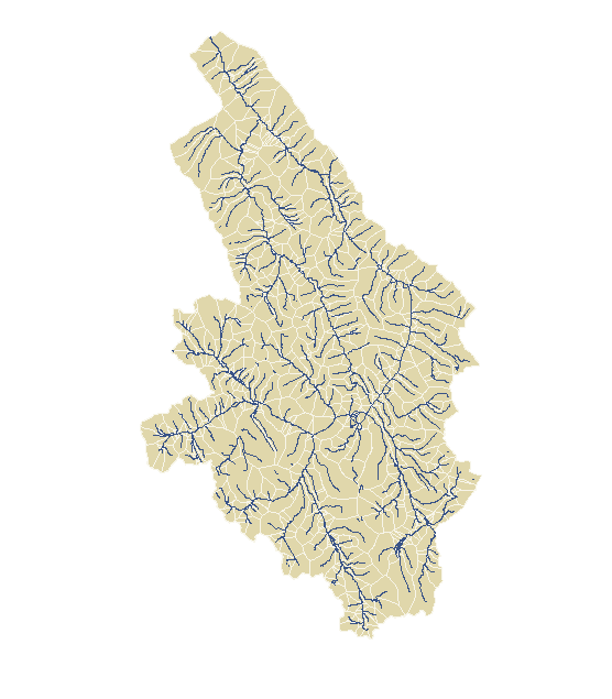
Reach contributing area (or RCA) polygons are used are pseudo-subunits to help delineate drainage basin boundaries.
# Load example data filename_strm <- system.file("extdata", "NHN_HN_NLFLOW_1.gpkg", package = "canadaNHN") strm <- sf::st_read(paste0(filename_strm), layer="NHN_HN_NLFLOW_1") strm <- sf::st_zm(strm) # Drop z geometry # Convert to local UTM zone strm <- sf::st_transform(strm, util_utm_zone(strm)) # Load basin boundary filename_basin <- system.file("extdata", "NHN_WORKUNIT_LIMIT_2.gpkg", package = "canadaNHN") basin <- sf::st_read(paste0(filename_basin), layer="NHN_WORKUNIT_LIMIT_2") # Recommended step: Run get_upstream_lines() first with the basin outlet this prevents network topology issues with isolated segments. # NHN Working unit outlet junction ID outlet_junction <- '310665e2e3dd4738b26b031a85d2bb19' strm_fix <- get_upstream_lines(strm = strm, jnid = outlet_junction) # RCA Polygons from NHN network rca <- generate_rca_polygons(basin = basin, strm = strm_fix, pt_density_m = 50) plot(sf::st_geometry(rca), col = "#e0d7ab", border = "#f7f5e9") plot(sf::st_geometry(strm), col = "#395387", add = TRUE)
Delineate Upstream Drainage Basin
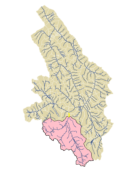
Delineate upstream drainage basin with reach contributing area (RCA) polygons (from previous step). Note that this methodology does not create perfect watershed boundaries and may not work well in steep terrain.
# Identify a target NHN junction ID for upstream delineation target_junction <- "c2ad6151e60a49dbabcb59d85eda4cba" watershed <- get_upstream_polygons( jnid = target_junction, strm = strm, rca = rca, # from previous step (above)... dissolve = TRUE) # View result plot(sf::st_geometry(watershed), col = "pink", add = TRUE) out_sl <- strm[strm$fromJunction == target_junction, ] plot(sf::st_geometry(strm), col = "#395387", add = TRUE) plot(sf::st_geometry(out_sl), add = TRUE, col = "yellow", lwd = 3)
Code of Conduct
Please note that the canadaNHN package is released with a Contributor Code of Conduct. By contributing to this project, you agree to abide by its terms.
