Water Withdrawals during Low Flow Conditions and System Capacit

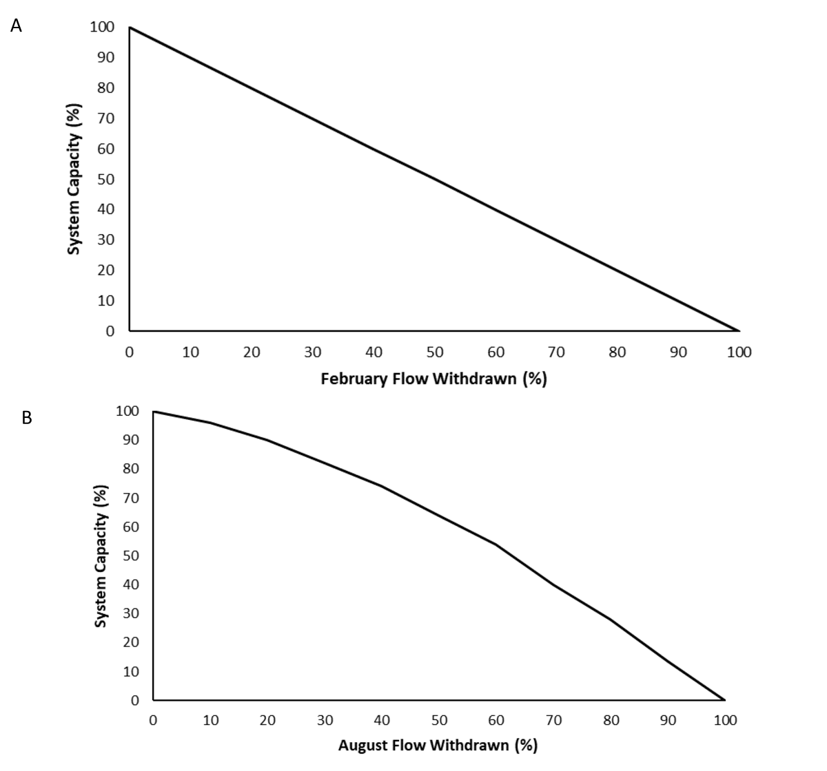
The effect of water withdrawals during February (winter) and August (summer) on the three native trout species was investigated using a multi-step analytical approach based on the low-flow habitat performance measures developed by Hatfield and Paul (2015). First, it was assumed there was a 1:1 relationship between the minimum available habitat (bottleneck effect) and the three trout species populations system capacity. To measure habitat, an index presented by Hatfield and Paul (2015) was used which: a) sets all flows >20% Mean Annual Discharge (MAD) to a habitat score of 1 (i.e., maximum suitability); b) has a habitat score of 0 at zero flow (i.e., no suitability); and, c) has a habitat score between 0 and 1 for flows between 0 and 20% MAD using a linear relation. This simple rating curve means that a flow of just under 20% MAD will score close to the maximum of 1, whereas a substantially lower flow will score proportionally less. The index was then used to determine the reduction in habitat scores from water withdrawals. Because withdrawals would have the greatest impact on the habitat score during low flows (i.e., < 20% MAD), percent withdrawal was determined for two periods of the year (August and February) and the lowest 10% of flows (i.e., Q90 or 90% exceedance flow) for these months. The approach was then applied to 37 rivers of varying size in Alberta that had year-round natural or naturalized (i.e., corrected for upstream water use) discharge and percent withdrawals ranging from 0–100% were modelled to assess the decrease in the habitat score from natural.
For February flow, all 37 rivers showed a similar linear response in the habitat score to water withdrawals. This average response was used as the basis for the stressor-response curve (Figure 1A). For August flows, the rivers showed a highly variable response in the habitat score to water withdrawals, ranging from linear (similar to February) to curvilinear with little initial response but increasing as withdrawals increased. The 75th percentile regression using a general additive model (Koenker 2017) was used to capture the curvilinear relationship (Figure 1B). The overall cumulative effects model only includes the season during which water withdrawals have the greatest effect on bull trout as physical habitat is assumed to limit populations by the minimum and not the combined product of February and August habitat.
As the Joe model accumulates cumulative effects multiplicatively (additive on a proportional scale), treating these two curves separately would inappropriately overemphasize the expected response. To overcome this issue, we treated February and August flow in the Joe model using a limiting factor approach. Simply, only the strongest, negative response from either the February and August stressor-response curves is used to calculate final system capacity. Anytime a watershed shows either February or August flow to be a hypothesized key driver, it must be acknowledged that the other stressor could be the driver given the collinearity

References Cited

Government of Alberta. 2024. Surface water withdrawal stressor-response function for Athabasca Rainbow Trout, Westslope Cutthroat Trout, and Bull Trout. Environment and Protected Area Native Trout Cumulative Effects Model.
Hatfield, T., and J. Bruce. 2000. Predicting salmonid habitat–flow relationships for
streams from Western North America. North American Journal of Fisheries Management 20:1005-1015.
Hatfield, T., and A.J. Paul. 2015. A comparison of desktop hydrologic methods for determining environmental flows. Canadian Water Resources Journal 40:303-318.
Koenker, R. 2017. quantreg: Quantile Regression. R package version 5.33. https://CRAN.R-project.org/package=quantreg
Rosenfeld, J.S., and R. Ptolemy. 2012. Modelling available habitat versus available energy flux: do PHABSIM applications that neglect prey abundance underestimate optimal flows for juvenile salmonids? Canadian Journal of Fisheries and Aquatic Sciences 69(12):1920-1934.
File Upload
Images
Stressor Response Chart
Mean Response
±1 Standard Deviation
Upper/Lower Limits